
Are you tired of struggling to make your Excel spreadsheets more visually appealing? Do you wish there was a simple way to highlight trends or direct attention to specific data points?
You’re in luck! Arrows can be your secret weapon in transforming a dull spreadsheet into a dynamic tool that captures attention and conveys information effectively. This guide will show you exactly how to add arrows in Excel, turning your data into a story that is easy to follow and understand.
By the time you finish reading, you’ll not only have mastered this skill but also enhanced your ability to communicate insights clearly and compellingly. Dive in now to discover the straightforward steps that can elevate your Excel game and impress your audience!
Inserting Basic Arrows
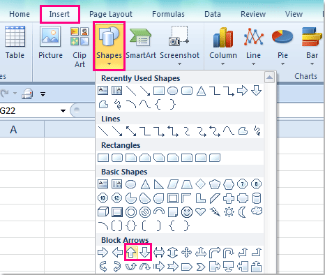
Open Excel and find the Insert Tabon the ribbon. Click it to see options. Choose Shapes. This gives many shapes to pick. Arrows are in this list. Click an arrow shape you like. Drag to place it in your worksheet.
Different arrow shapes offer different styles. Long arrows, short arrows, curved arrows. Pick one that fits your need. Shapes can be resized. Drag the corners to make them bigger or smaller. Change colors by right-clicking and choosing Format Shape. Choose the color you want. Make arrows look nice and clear.
Formatting Arrows
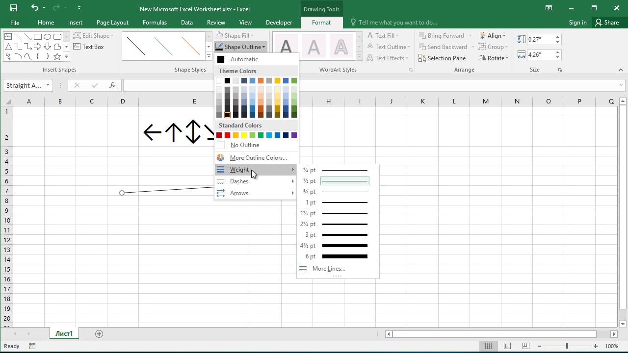
Choose your arrow on the worksheet. Right-click on it. Find Format Shape. Click it. Look for the Fill & Line tab. Select Line Color. Pick a new color. Watch your arrow change. Simple and fun.
Click your arrow. Find the small square at the arrow’s end. Drag it to make the arrow bigger or smaller. Easy to adjust. Try different sizes. Make it fit your needs.
Click the arrow you want to rotate. Find the circular arrow above it. Drag this circle to rotate. Move it left or right. Rotate to any angle. Make arrows point anywhere. It’s quick and easy.
Using Arrow Symbols
Open Excel. Click on the Inserttab. Find the Symbolicon. It’s usually on the right side. Click on it. A new box opens. This is the Symbol Menu. You can see many symbols here. Look at the top. You’ll see Fontand Subsetoptions. These help find symbols fast. Use them to locate arrows.
Different arrows show different meanings. Pick the right one for your task. In the Symbol Menu, scroll down to find arrows. There are many types. Short arrows. Long arrows. Curved arrows. Choose the one you need. Click on it once. Then click Insert. The arrow appears in your Excel sheet.

Credit: trumpexcel.com
Creating Custom Arrows
Excel lets you make arrows using shapes. First, go to the Inserttab. Choose Shapes. Pick a line shape. Draw it on your sheet. Add a triangle shape at the end. Place it where the line ends. Now you have an arrow. You can change the color. You can make it bigger or smaller. Adjust it to fit your needs.
Drawing tools help create arrows easily. Start by clicking on the Inserttab. Select Shapes. Choose an arrow shape. Drag it onto your sheet. You can adjust its size. Change its color using the Formattab. Make sure it points where you want. Arrows can show direction. They make data easy to understand.
Adding Arrows In Charts
Arrows help show data trends. First, choose the chart type. Line charts are great for trends. Then, click on the chart. Select the “Insert” tab. Now, choose “Shapes” and pick an arrow. Drag the arrow to where you want it. Make sure it points the right way. You can resize it by dragging the corners.
To make arrows look good, use the Format option. Click on the arrow. Choose “Shape Format” from the menu. Change the color to match your chart. You can also adjust the arrow style. Thick or thin lines? It’s your choice. Add some effects like shadow for a cool look. Always check if the arrow fits the chart’s style.
Using Conditional Formatting
Credit: www.extendoffice.com
Conditional Formatting helps show trends in data. Select the cells you want to format. Click on “Conditional Formatting” in the toolbar. Choose “New Rule.” This step is key to setting up your data display.
Choose “Format Style” as Icon Sets. Pick the arrow style you like. Arrows can point up, down, or sideways. They make data trends easy to see.
Arrows show if numbers go up or down. Green arrows show a rise. Red arrows mean a drop. Yellow arrows show no change. These colors help understand data fast.
Adjust the rules for the arrows. Set values for each arrow. This fine-tunes how data is shown. Understanding data becomes simple with arrows.
Troubleshooting Common Issues
Need to insert arrows in Excel? Select the ‘Insert’ tab, click ‘Shapes’, and choose the arrow style. Adjust its size and direction using the handles. Arrows help highlight data flow or trends.
Fixing Arrow Display Problems
Arrows sometimes don’t show up in Excel. This can be due to hidden rows or columns. Make sure everything is visible. Check if arrow color matches the background. Arrows may blend in and become invisible. Zoom settings can also affect arrow visibility. Adjust zoom to see if arrows appear. Try refreshing the page to solve display issues.
Resolving Formatting Errors
Formatting errors can mess up arrow appearance. Ensure correct cell formatting. Sometimes wrong formats hide arrows. Check if arrow size is set properly. Small arrows might be hard to see. Adjust size to make them visible. Alignment issues can also cause problems. Make sure arrows are properly aligned within cells. This ensures they look correct.
Credit: www.youtube.com
Frequently Asked Questions
How Do I Insert Arrows In Excel?
To insert arrows in Excel, go to the “Insert” tab. Click on “Shapes” and select the arrow style you prefer. Click and drag on your worksheet to draw the arrow. You can customize it using the “Format” tab for color, size, and direction adjustments.
Can I Add Arrow Keys In Excel Cells?
You can’t insert arrow keys directly into cells. However, you can use the “Symbols” feature. Go to the “Insert” tab, click “Symbols,” and search for arrow characters. Insert them into your cell as needed for visual representation.
How To Change Arrow Direction In Excel?
To change the arrow’s direction, click on the arrow to select it. Use the rotation handle at the top of the arrow to rotate it. Alternatively, go to the “Format” tab and use the “Rotate” option for precise adjustments.
Are There Shortcut Keys For Drawing Arrows?
Excel doesn’t have direct shortcut keys for drawing arrows. However, you can use “Alt” codes for arrow symbols. For example, press “Alt” + “26” to insert an upward arrow. These codes work only with the numeric keypad.
Conclusion
Adding arrows in Excel is now easy. Just follow the steps. It helps highlight important data. Arrows make your spreadsheets clear. They guide viewers quickly. Practice using them regularly. You’ll improve your Excel skills. Arrows add a professional touch. They enhance data presentation.
Keep exploring Excel features. They offer more ways to improve your work. Happy arrow adding! Excel is a useful tool. Make the most of it. Enjoy creating better spreadsheets. Your data deserves the best presentation.